Building the Largest Clinical Brain Embedding Model

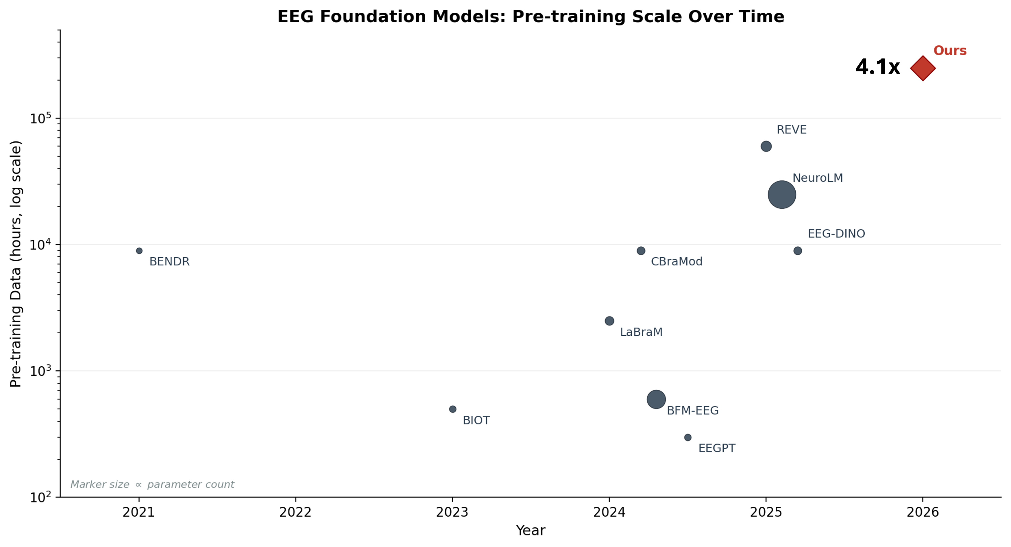
We trained a masked autoencoder on 250,000 hours of clinical EEG, roughly 31 million 30-second epochs from 8,352 patients at the Swiss Epilepsy Center. The result is EPI-250k, currently the largest self-supervised model trained on clinical EEG data ¹.

What came before

The EEG foundation model landscape has grown quickly. BENDR (2021) adapted wav2vec to the Temple University Hospital corpus. LaBraM (2024) aggregated ~2,500 hours from 20 research datasets with a VQ-VAE tokenizer. REVE (2025) scaled to 60,000 hours from 92 datasets using a modified MAE. On the clinical side, BioSerenity trained on 4,000 hours of proprietary data, the largest single-source clinical model before ours.

Most of these models share a pattern: fairly strong neuroscience priors baked into the architecture (montage-specific embeddings, hand-crafted frequency features, task-specific heads) and evaluation on a fragmented set of benchmarks that makes comparison difficult. The clinical models that exist are small. The large models train mostly on research or mixed datasets.

Sutton's Bitter Lesson ² is the starting point. In every domain (chess, Go, speech, vision) general methods that leverage computation have eventually beaten approaches that encode human knowledge. A good model should learn features on its own from large amounts of data with as little inductive bias as possible. That was our thesis going in: a standard masked autoencoder (Hiera ³) that masks some % of input patches and learns to reconstruct the missing regions, minimal preprocessing, and a lot of clinical data.

The data

The Swiss Epilepsy Center (Klinik Lengg) has been recording clinical EEG since 2000.

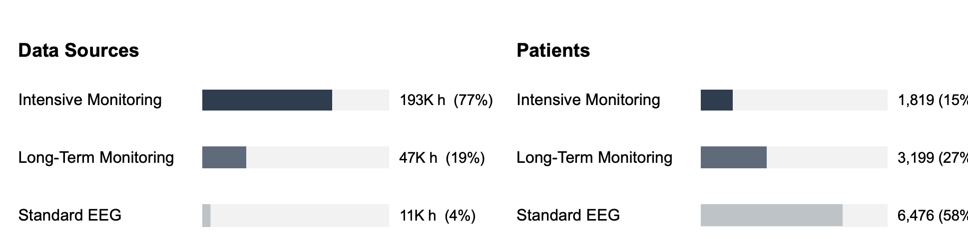
The raw archive includes intensive monitoring recordings (multi-day, continuous), routine outpatient EEGs, and long-term monitoring sessions. All in proprietary hospital formats (Nicolet .e and Micromed .TRC), neither of which has a public specification ⁴. The .e format was the dominant standard for clinical EEG until recently, when most centers started migrating to Micromed. We wrote modified versions of the Neo library's file readers. The critical bottleneck was that the original readers used memory-mapped reads that triggered many small network round-trips on the hospital filesystem. We replaced these with direct buffered reads, reducing each chunk load to a single network operation. The result: 1.73x average speedup on Nicolet files (up to 3.23x on large files), 1.15x on Micromed. Not glamorous, but on a 4-5 week pipeline this saved days.

The preprocessing pipeline takes a raw recording and produces training-ready epochs through 10 stages. The interesting ones: reading proprietary formats via modified Neo readers with buffered I/O (1.3-3x faster on network filesystems), extracting bilingual German/English clinical annotations (Nicolet tracks the annotating clinician, Micromed requires decoding from a binary format), automatic sleep staging via the GSSC neural network, and clustering events against a taxonomy of 200+ clinical keywords into 5 categories and ~56 subcategories. The rest is standard signal conditioning (bandpass, notch, resampling to 250 Hz), segmentation into 30-second epochs, channel averaging from 19 electrodes to 8 regional groups, quality scoring, and serialization into WebDataset tar shards.

We spent roughly four to five weeks running this pipeline locally on a workstation with two GPUs. The GPUs ran in a round-robin setup: one dedicated to sleep staging inference (the GSSC model), the other handling signal preprocessing and spectrogram computation. The pipeline tracked completed files by SHA-256 hash in a CSV resume log and could be restarted at any point without reprocessing. About 95% of files processed successfully. The 5% that failed were corrupted headers, unreadable proprietary encodings, or segments too short to extract 10 valid epochs from.

The output: 31.6 million epochs in ~25,000 tar shards, transferred to the Swiss National Supercomputing Centre (CSCS) via Globus for training on the Alps supercomputer.

Making it fast: flash-eeg

Standard EEG tools are written in Python and process one recording at a time. The problem is visible in a torch profiler trace of the baseline SciPy STFT:

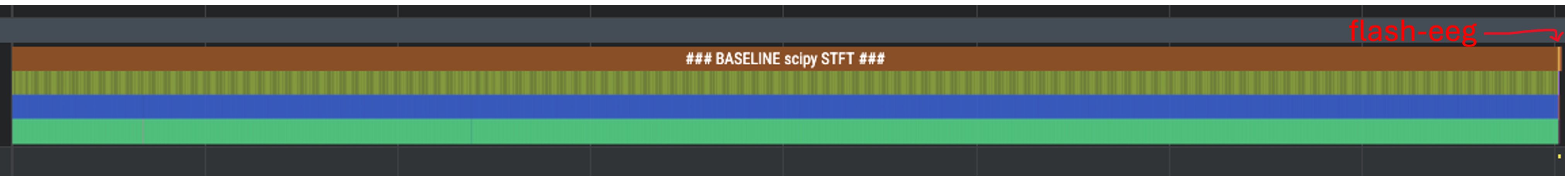
Torch profiler trace on a batch of 1,024 samples: SciPy STFT takes 3,378 ms (the long bar of repeated sequential CPU calls). flash-eeg takes 7.4 ms (the red label on the right, so thin it's barely visible). Same output. This was measured on an H100. On GH200 the numbers are slightly different but the ratio holds.

We built flash-eeg ⁵, an open-source library that reimplements common electrophysiology transforms as fused, GPU-accelerated PyTorch operations.

Under the hood, everything is vectorized tensor operations with no Python loops, so torch.compile can trace the full computation into a single fused kernel. The WPLI connectivity does a batched FFT across all channels, computes cross-spectral density via an outer product, and extracts all 8 frequency bands simultaneously using precomputed DPSS tapers registered as buffers. No iteration over channel pairs, no iteration over bands.

Compilation mode matters: max-autotune for fixed 30-second inputs (best throughput, auto-tunes CUDA kernel configs), reduce-overhead with dynamic=True for variable-length training where we randomly subsample to 30s, 15s, 10s, or 5s segments.

Benchmarks on a GH200 at batch size 2048:

Representation	CPU baseline	GPU compiled	Speedup
Spectrogram (vs. SciPy)	14.85s	0.012s	1,200x
Temporal matrix	12.86s	0.002s	7,700x
WPLI Connectivity (vs. MNE)	142.00s	0.002s	70,000x

The spectrogram speedup (1,200x) is the representative number for most use cases. The 70,000x on connectivity is real but the gap is so large because MNE's WPLI iterates over every channel pair (8x8 = 64) and every frequency band (8) in Python, launching separate NumPy operations for each. That's 512 sequential Python-level operations per epoch, per batch element. Our implementation does a single batched FFT, a single vectorized outer product for cross-spectral density, and a single gather per band. The entire computation is one CUDA graph.

The model

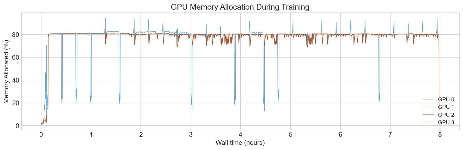
Training ran on CSCS Alps (GH200 nodes, 4-32 GPUs) with bfloat16 mixed precision and FlashAttention via F.scaled_dot_product_attention. We train models from 52M encoder parameters, to 214M. We use Hiera with a hierarchical 4-stage encoder (embedding dims 96 to 768). The final EPI-250k model trained in just under 3 days.

Optimizer. We use a dual-optimizer strategy.

Muon ⁶ orthogonalizes gradient momentum via Newton-Schulz iteration, which keeps weight matrices well-conditioned throughout training. The key practical benefit is that its learning rate transfers across batch sizes thanks to built-in muP scaling - one less hyperparameter to sweep when moving between GPU counts. But Muon only operates on 2D weight matrices. Embeddings, biases, and layer norm parameters are 1D tensors, and for those you still need a standard optimizer. We use AdamW at a separate learning rate (3e-4 vs. Muon's 0.02).

The interesting thing about Muon is where the advantage shows up. In our ablation comparing Muon vs. AdamW on the same architecture, the training loss curves look similar (Muon actually starts higher because of its different learning rate regime):

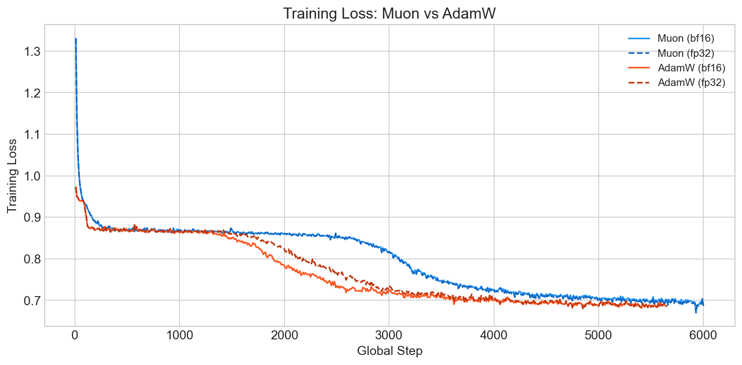
But Muon converges noticeably faster and reaches a lower final val loss:

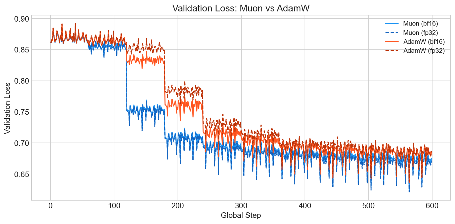
This is consistent with what others have observed ⁷: Muon's spectral-norm steepest descent appears to find better-generalizing solutions rather than simply optimizing the training objective faster. The orthogonalization acts as an implicit regularizer that doesn't show up in training loss but matters for downstream performance.

One thing worth knowing: fused optimizers (which both Muon and AdamW support) are incompatible with gradient clipping. If you enable both, you get silent numerical issues: no error, just degraded training. The code disables clipping automatically when fused=True.

Channel stacking. The model needs to see 8 EEG channels simultaneously. We stack them as "color channels": the input tensor is [B, 8, 224, 224] and the patch embedder has access to all channels at every spatial position. We don't change the patch size or model configuration because the signal is stationary at 30 seconds, so there's no need for the model to treat channels differently from how a vision model treats RGB.

For the 3D video variant, each channel becomes a "frame": [B, n_repr, 8, H, W]. The idea came from staring at a pre-sliced block of cheese at my parents' breakfast table:

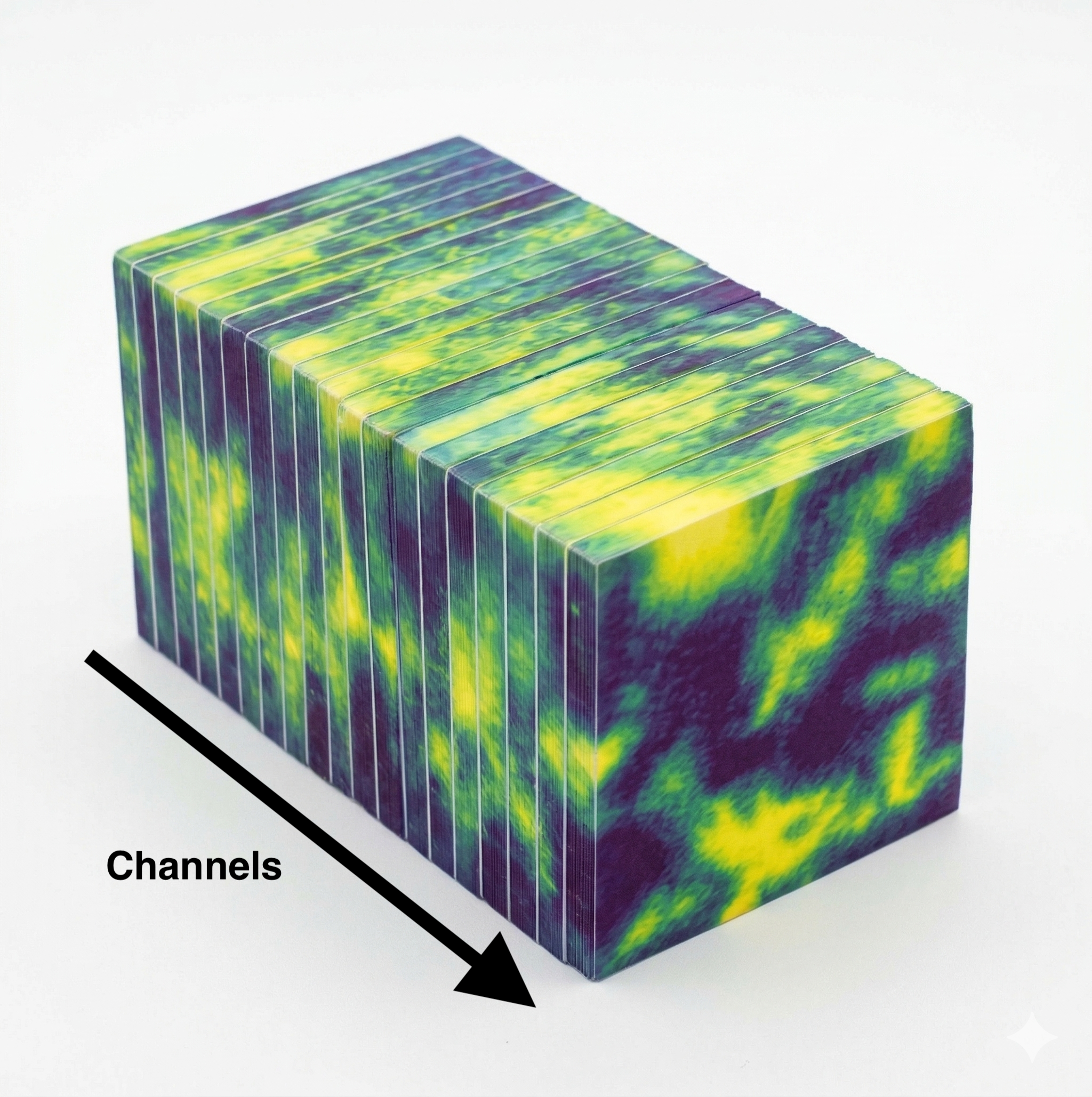
Each slice is a channel. Look at individual slices for spatial features within a channel, or across the block for cross-channel relationships. The 3D patch embedding uses a 1x7x7 kernel with 1x4x4 stride, no pooling across the channel axis initially, preserving channel independence in the early layers. With 3D inputs we push the mask ratio from 0.6 to 0.9, following VideoMAE's finding that higher masking forces stronger spatiotemporal reasoning.

What the model learned

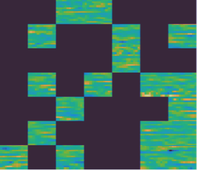
Here is what the MAE reconstruction looks like on temporal matrices. When the input signal has clear structure (consistent patterns, recognizable waveforms), the model reconstructs masked regions well:

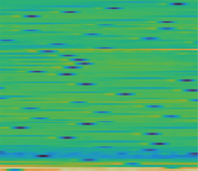
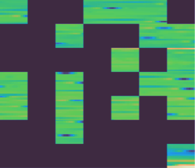
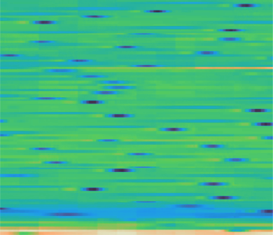
Left: original. Center: masked (60% of patches removed). Right: reconstruction.

When the signal is noisy or unpredictable (distorted, random-looking EEG), the model struggles to fill in the masked regions:

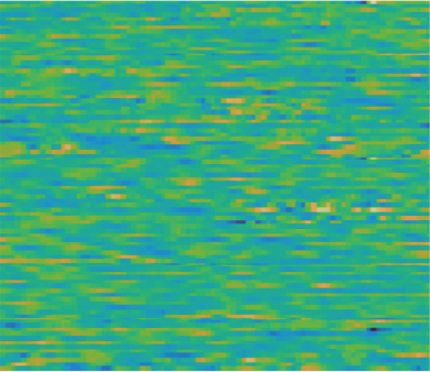
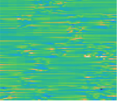
This makes sense: if the signal itself has little predictable structure, there is less for the model to learn from. The good news is that clinically relevant patterns (seizures, spikes, sleep spindles) tend to have strong, recognizable structure.

Scaling

We ran scaling experiments across 4 orders of magnitude: 10 hours to 100,000 hours of data, with models from 28M to 214M parameters. The compute budget spans 0.01 to 155 PetaFLOPs.

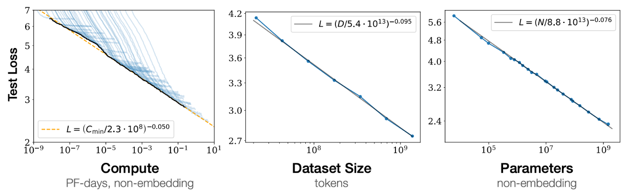
For context, Kaplan et al.'s original scaling laws for language show clean power laws over many orders of magnitude:

And here is ours for clinical EEG:

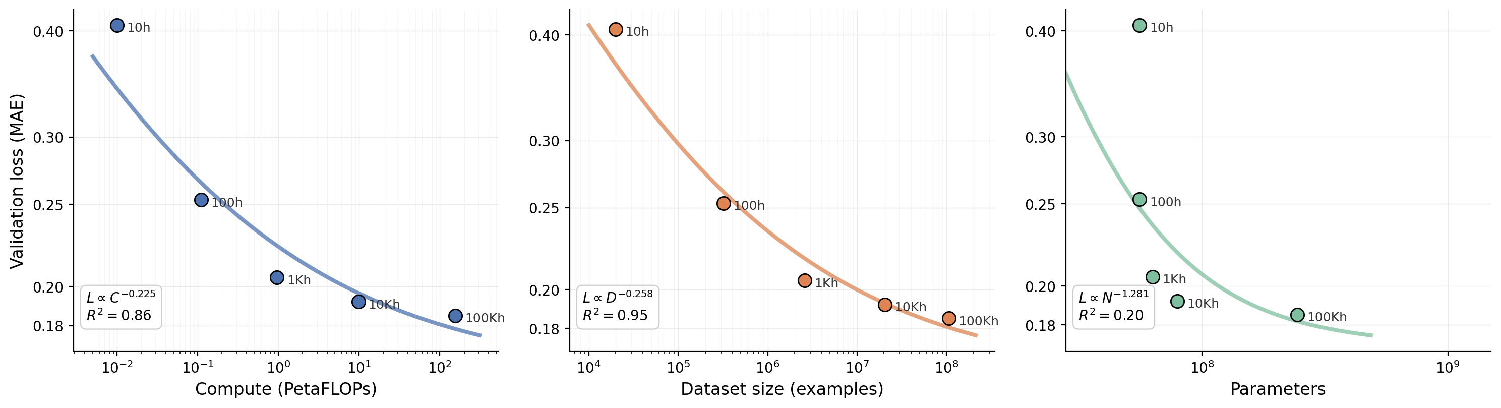
Fitting a power law to our data gives L ∝ C^(-0.225) for compute (R² = 0.86) and L ∝ D^(-0.258) for dataset size (R² = 0.95). At first glance these exponents look much steeper than language (Kaplan's α_C ≈ 0.05) or vision (α_C ≈ 0.07). But the curves tell a different story than the exponents alone: the loss flattens out visibly as we push past 1,000 hours. The power law fit captures this because the early points (10h, 100h) dominate the slope, but each additional order of magnitude buys less and less.

This is a concrete picture of diminishing returns for a bounded modality. In language, new topics and new ways of expressing them appear indefinitely; the power law keeps going because the data keeps surprising the model. In clinical EEG, the cortex draws on a limited repertoire of oscillatory states, and volume conduction through the skull constrains what's observable. The annotation taxonomy at the Swiss Epilepsy Center covers roughly 40 categories. After enough hours from one hospital, the model has seen most of what the modality can show.

Why EEG scales "better" at first. Sharma & Kaplan (2020) ⁸ showed that scaling exponents are inversely proportional to the intrinsic dimension of the data manifold: α ~ 4/d. A steeper early exponent implies the data lives on a lower-dimensional manifold. This is plausible for clinical EEG. Natural images have intrinsic dimensions estimated at 26-43 for ImageNet ⁹. EEG spectrograms and temporal matrices are generated by a far more constrained physical process: a handful of oscillatory rhythms (delta, theta, alpha, beta, gamma) mixing across ~20 channels, modulated by a limited set of clinical states. There are no dogs, no faces, no compositional scene semantics. Just continuous oscillatory patterns governed by relatively simple electrophysiology. Early on, compute is enormously productive because the model is carving up a low-dimensional manifold.

Why it flattens. The same property that makes EEG scale fast makes it saturate. The low-dimensional manifold is resolved quickly. Once most of it has been mapped, additional compute has nothing new to learn. Natural image pretraining doesn't hit this wall because the space of possible natural images is vast and compositional, with discrete semantic structure (the world is composed of distinct objects, parts, and categories) that provides reusable "anchor concepts" for transfer. EEG lacks that structure. The representation scales beautifully on reconstruction loss early, but produces a latent space that is smooth and semantically flat, good at interpolating between brain states but lacking the discrete hooks that make representations transferable to classification. At some point the irreducible loss floor is low (less entropy in the data-generating process), there is simply less left to reduce.

Results

With patient-level train/test splits (no patient appears in both splits) and linear probes on frozen EPI embeddings, the model achieves state-of-the-art on seizure detection: Cohen's κ = 0.85 on recordings with clear ictal events, compared to expert-to-expert agreement of κ = 0.58 ¹⁰. Beats every published EEG model on our 10 private clinical tasks and most public benchmarks.

A side effect we didn't expect: state-of-the-art on Parkinson's detection. Roughly half of our training data comes from intensive monitoring recordings that span entire nights. The model picked up sleep features (spindles, K-complexes, stage transitions) that correlate with neurodegenerative markers clinicians use to distinguish Parkinson's from healthy controls. We didn't train for this. The sleep structure was just there in the data.

What we learned

A few lessons that generalized for us:

• Use established, well-tested infrastructure as early as possible. Flash Attention, and pretty much everything NVIDIA ships.

• Throughput is everything. If your model is general enough and you have enough throughput, it will learn. Optimize for keeping the GPUs fed before optimizing anything about the model itself.

• Distribution collapse, or diversity collapse, is a real thing. Bounded modalities saturate faster than you expect, and more volume from the same source stops helping.

• Don't train the largest model by default. Do iterative experiments in bigger and bigger containers, then extrapolate to the final run.

Footnotes

1. Paper currently being written. Link will be added upon publication. ↩

2. Richard Sutton, The Bitter Lesson, 2019. "The biggest lesson that can be read from 70 years of AI research is that general methods that leverage computation are ultimately the most effective." ↩

3. Ryali et al., Hiera: A Hierarchical Vision Transformer without the Bells-and-Whistles, 2023. Chosen for its hierarchical multi-scale structure and native 2D/3D support. ↩

4. We modified Python Neo library readers with buffered I/O, reducing network round trips by 2 to 3 orders of magnitude on the hospital network filesystem. ↩

5. flash-eeg is open source. Supports spectrogram, Morlet wavelet, WPLI connectivity, signal-to-image reshaping, and FFT bandpass filtering. Automatic torch.compile on A100/H100/H200/GH200. Float16/bfloat16 compatible. ↩

6. Keller Jordan, Muon optimizer, 2024. Theoretical grounding as steepest descent under the spectral norm by Jeremy Bernstein. Originally developed in the modded-nanogpt speedrun project. ↩

7. Muon achieved ~2x convergence speedup over AdamW at GPT-2 scale in the modded-nanogpt benchmark. The advantage manifests more in validation/downstream performance than training loss, suggesting better generalization rather than faster optimization. ↩

8. Sharma & Kaplan, A Neural Scaling Law from the Dimension of the Data Manifold, 2020. ↩

9. Pope et al., The Intrinsic Dimension of Images and Its Impact on Learning, ICLR 2021. ↩

10. Inter-rater agreement varies by task: general EEG interpretation κ=0.44, interictal epileptiform discharge identification κ=0.49, seizure annotation κ=0.58. ↩